“Hummingbird” is the name of the new search platform that Google is using as of September 2013, the name comes from being “precise and fast” and is designed to better focus on the meaning behind the words. Read ourGoogle Hummingbird FAQ here.
Google has a new search algorithm, the system it uses to sort through all the information it has when you search and come back with answers. It’s called “Hummingbird” and below, what we know about it so far.
What’s a “search algorithm?”
That’s a technical term for what you can think of as a recipe that Google uses to sort through the billions of web pages and other information it has, in order to return what it believes are the best answers.
Important notice for users of Office 2003 To continue receiving security updates for Office, make sure you're running Office 2003 Service Pack 3 (SP3).
The support for Office 2003 ends April 8, 2014. If you’re running
Office 2003 after support ends, to receive all important security
updates for Office, you need to upgrade to a later version such as
Office 365 or Office 2013. For more information, see Support is ending for Office 2003.
1. Tell me about FI Organizational structure? Ans: Client
|
Operating Concern
|
Controlling area1 Controlling Area
2
|
Co. Code 1 Co. Code 2
|
Bus area 1 Bus area2 Bus Area3 Bus Area 4
2. How many Normal and Special periods will be there in fiscal year,
why do u use special periods? Ans: 12 Normal posting period and 4 special periods are in the fiscal
year which can be used for posting tax and audit adjustments to a closed
fiscal year.
3.Where do you open and close periods? Ans: PPV is used to open and close the periods based on a/c types considering
GL Accounts. Tr. Code. OB52.
4.What do you enter in Company code Global settings? Ans: 4 digit Alphanumeric key.
Name of the company
City
Country
Currency
Language
Address
What are the frequently asked
questions on SAP FICO Interview Questions? 1. What is chart of account? What is the relevance of defining chart
of account?
A. It is the top level financial structure, contains the GL Accounts
we define the all the accounts and one chart of accounts assign to company
code and one chart of accounts will assign to many company codes . It is
list of Gl accounts and it contains account no , account name, language,
length, cost element, blocking information that controls the how an account
functions and how a gl account created in company code . COA Key.
2. What is account group? What does it control?
A. IT determines the which fields you need to configure on the GL master
record. It is necessary to have at least 2, one for B/S and another one
for P&L accounts. It controls the number ranges of GL. The Status fields
of the master record of GL Belong to company code area.
3. What is posting key? What is its role?
A. It controls the line item of GL entry debit and credit.
4. What is business area?
A. Organizational unit of external accounting that corresponds to a
specific business segment or area of responsibility in a company. Financial
statements can be created for business areas for internal purposes. They
are primarily used to facilitate external segment reporting across company
codes covering the main operation of a company (product line, Branches).
The Business area may be the branch of the company or product lines it
deals with
5. While defining chart of account, there is field "manual
creaation of cost element" and "automatic creation of cost element", what
is it? A. Generally when ever we are creating cost elements we can create
some of exependitures manually some automatically so we can create manually
cost elements in defining chart of accounts.
6. After creating a customer/vendor, how can we check that under
which account group we have configured this customer/vendor?
A. We can check through customer group and vendor group it was created
by ours when we are creating vendor and customer groups.
Six Sigma aims to define the causes of defects, measure those
defects, and analyze them so that they can be reduced.We will consider
five specific types of analysis that will help to promote the goals of
the project. These are source, process, data, resource, and
communication analysis. Now we will see them in detail:
1. Source Analysis:
This is also called root cause analysis and attempts to find defects
that are derived from the sources of information or work generation.
After finding the root cause of the problem, attempts are made to
resolve the problem before we expect to eliminate defects from the
product.
THE THREE STEPS TO ROOT CAUSE ANALYSIS
The open step: During this phase of root cause analysis,
the project team brainstorms all the possible explanations for current
sigma performance.
The narrow step: During this phase, the project team narrows the list of possible explanations for current sigma performance.
The close step: During this phase, the project team validates the narrowed list of explanations that explain sigma performance.
2. Process Analysis:
Analyze the numbers to find out how well or poorly the processes are
working, compared to what's possible and what the competition is doing.
Process analysis includes creating a more detailed process map and
analyzing the more detailed map for where the greatest inefficiencies
exist.
The source analysis is often difficult to distinguish from process
analysis.The process refers to the precise movement of materials,
information, or requests from one place to another.
During Measure Phase the overall performance of the Core Business Process is measured.
There are three important part of Measure Phase.
(1) Data Collection Plan and Data Collection
A data collection plan is prepared to collect required data. This
plan includes what type of data needs to be collected, what are the
sources of data etc., The reason to collect data is to identify areas
where current processes need to be improved.
You collect data from three primary sources: input, process, and output.
The input source is where the process is generated.
Process data refers to tests of efficiency: the time
requirements, cost, value, defects or errors, and labor spent on the
process.
Output is a measurement of efficiency.
(2) Data evaluation:
At this stage, collected data is evaluated and sigma is calculated. This gives approximate number of defects.
A Six Sigma defect is defined as anything outside of customer specifications.
A Six Sigma opportunity is the total quantity of chances for a defect.
First we calculate Defects Per Million Opportunities (DPMO) and based on that a Sigma is decided from a predefined table:
Number of defects
DPMO =------------------------------------------- x 1,000,000Number of Units x Number of opportunities
As stated above, here Number for defects is total number of
defects found, Number of Units is the number of units produced and
number of opportunities means the number of ways to generate defects.
For example: The food ordering delivery project team examines 50 deliveries and finds out the following:
Delivery is not on time (13)
Ordered food is not according to the order (3)
Food is not fresh (0)
So now DPMO will be as follows:
13+3
DPMO =----------- x 1,000,000=106,666.750 x 3
According to the Yield to Sigma Conversion Table given below
106,666.7 defects per million opportunities is equivalent to a sigma
performance of between 2.7 and 2.8.
This is the method used for measuring results as we proceed through a
project. This beginning point enables us to locate the cause and effect
of those processes and to seek defect point so that the procedure can
be improved.
There are five high-level steps in the application of Six Sigma to
improve the quality of output. The first step is Define. During define
phase following four major tasks are undertaken.
(1) Project team is Formed:
Perform two activities:
Determine who needs to be on the team.
What roles each person will perform
Picking the right team members can be a difficult decision,
especially if a project involves a large number of departments. In such
projects, it could be wise to break them down into smaller pieces and
work toward completion of a series of phased projects
(2) Document customers Core Business Processes:
Every project has customers. A customer is the recipient of the
product or service of the process targeted for improvement. Every
customer has one or multiple needs from his or her supplier. For each
need provided for, there are requirements for the need. The requirements
are the characteristics of the need that determine whether the customer
is happy with the product or service provided. So document customer
needs and related requirements.
A set of business processes is documented. These processes will be
executed to meet customer's requirements and to resolve their Critical
to Quality issues.
(3) Develop a project charter:
This is a document that names the project, summarizes the project by
explaining the business case in a brief statement, and lists the project
scope and goals. A project charter can have following components
DMAIC: refers to a data-driven quality strategy for
improving processes. This methodology is used to improve an existing
business process.
DMADV: refers to a data-driven quality strategy for
designing products & processes. This methodology is used to create
new product designs or process designs in such a way that it results in a
more predictable, mature and defect free performance.
There is one more methodology called DFSS - Design For Six
Sigma. DFSS is a data-driven quality strategy for designing design or
re-design a product or service from the ground up.
Sometimes a DMAIC project may turn into a DFSS project because the
process in question requires complete redesign to bring about the
desired degree of improvement.
DMAIC Methodology:
This methodology consists of following five steps. Define --> Measure --> Analyze --> Improve -->Control
Define : Define the Problem or Project Goals that needs to be addressed.
Measure: Measure the problem and process from which it was produced.
Analyze: Analyze data & process to determine root causes of defects and opportunities.
Improve: Improve the process by finding solutions to fix, diminish, and prevent future problems.
Control: Implement, Control, and Sustain the improvements solutions to keep the process on the new course.
In the subsequent session we will give complete detail of DMAIC Methodology.
DMADV Methodology:
This methodology consists of following five steps. Define --> Measure --> Analyze --> Design -->Verify
Define : Define the Problem or Project Goals that needs to be addressed.
Measure: Measure and determine customers needs and specifications.
Analyze: Analyze the process for meet the customer needs.
Design: Design a process that will meet customers needs.
Verify: Verify the design performance and ability to meet customer needs.
The starting point in gearing up for a Six Sigma is to verify that
you are ready to embrace a change that says "There is a better way
to run your Organization".
There are number of essential questions and facts you will have to consider in making a readiness assessment:
Is the strategic course clear for the company ?
Is the business healthy enough to meet the expectations of analysts and investors ?
Is there a strong theme or vision for the future of the organization that is well understood and consistently communicated ?
If the organization good at responding effectively and efficiently to new circumstances ?
Evaluating current overall business results.
Evaluating how effectively do we focus on and meet customers requirements ?
Evaluating how effectively are we operating ?
How effective are your current improvement and change management systems ?
How well are your cross functional processes managed ?
What other change efforts or activities might conflict with or support Six Sigma initiative ?
Six Sigma demands investments. If you can not make a solid case for future or current return then it may be better to stay away.
If you already have in place a strong, effective, performance and process improvement offer then why do you need Six Sigma ?
There could be many questions to be answered to have an extensive
assessment before deciding if you should go for Six Sigma or not. This
may need time and a thorough consultation with Six Sigma Experts to
take a better decision.
The Cost of Six Sigma Implementation:
Some of the most important Six Sigma budget items can include the followings:
Direct Payroll for the individuals dedicated to the effort full time.
Indirect Payroll for the time devoted by executives, team
members, process owners and others involved in activities like data
gathering and measurement.
Training and Consultation fee to teach people Six Sigma Skills and getting advice on how to make effort successful.
Under a Six Sigma program, members of an organization are assigned
specific roles to play, each with a title. This highly structured
format is necessary in order to implement Six Sigma throughout the
organization.
There are seven specific responsibilities or "role areas" in the Six Sigma program. These are:
Leadership:
A leadership team or council defines the goals and objectives in the
Six Sigma process. Just as a corporate leader sets a tone and course to
achieve an objective, the Six Sigma council sets out the goals to be met
by the team. Here is the list of leadership Council Responsibilities,
Define the purpose the Six Sigma Program.
Explain how the result is going to benefit the customer.
Set a schedule for work and interim deadlines.
Develop a means for review and oversight.
Support team members and defend established positions.
Sponsor:
Six Sigma sponsor are high-level individuals who understand Six Sigma
and are committed to its success. The individual in the sponsor role
acts as a problem solver for the ongoing Six Sigma project. Six Sigma
will be lead by a full-time, high-level champion, such as an Executive
Vice President.
Sponsors are owners of processes and systems who help initiate and
coordinate Six Sigma improvement activities in their areas of
responsibilities.
Lean Six Sigma is a methodology for quality improvement that has been around for many years in the industrial environment.
GE
under Jack Welch, was a leading proponent of Lean Six Sigma globally.
Genpact (at that time known as GE Capital International Services) was
the first service provider in the world to apply this methodology at
scale for business processes making this practice a tremendous success.
Lean Six Sigma permeates what we do and is highly visible in our operations, people, processes, and leadership direction.
We
take a different approach to implementation of Lean Six Sigma, going
beyond the scope of the contract to take a comprehensive
upstream/downstream view, which extends our impact on client’s
businesses.
There are three key elements of Six Sigma Process Improvement.
Customers
Processes
Employees
The Customer:
Customers define quality. They expect performance, reliability,
competitive prices, on-time delivery, service, clear and correct
transaction processing and more.
Today, Delighting a customer is a necessity. Because if we don't do it, someone else will!
The Processes:
Defining Processes and defining Metrics and Measures for Processes is the key element of Six Sigma.
Quality requires to look at a business from the customer's
perspective, In other words, we must look at defined processes from the
outside-in.
By understanding the transaction lifecycle from the customer's needs
and processes, we can discover what they are seeing and feeling. This
will give a chance to identify week area with in a process and then we
can improve them.
To watch calculations results immediately:
1. Select range of cells containing numeric data.
2. Select the Status Bar and right-click to open Status Bar shortcut menu.
Six functions are available:
Average, Count, Numerical Count, Minimum, Maximum and Sum
Results appear at the right of each formula in the shortcut menu.
Or
Check all or any other formulas you want to watch the result calculation for in the Status Bar.
The following articles are available for the 'Worksheet Functions' topic. Click the article's title (shown in bold) to see the associated article.
Calculating Fractions of Years When
working with dates and the relationship between dates, Excel provides a
variety of worksheet functions that may prove helpful. One such
function is YEARFRAC, which allows you to calculate what fraction of a
year is represented by the number of days between two dates.
Converting Strings to Numbers When
working with data in a macro, there are two broad categories you can
manipulate: numbers and text. Sometimes you need to convert information
from one category (data type) to another. Here is how you convert text
to numbers.
Converting to Hexadecimal Excel
allows you to easily convert values from decimal to other numbering
systems, such as hexadecimal. This tip explains how to use the DEC2HEX
worksheet function.
Converting to Octal If
you need to do some work in the base-8 numbering system (octal), you'll
love two worksheet functions provided by Excel for this purpose. These
functions allow you to convert values to octal and convert them back
again.
Counting Displayed Cells When
you filter data, Excel displays only a portion of what is really in a
worksheet. If you want to count the number of cells that are displayed
after filtering, then you'll want to explore the techniques in this tip.
Counting Unique Values with Functions Using
Excel to maintain lists of information is not unusual. When working
with the list you may need to determine how many unique values it
contains. This tip shows you how.
Functions Within Functions Functions
are the heart of Excel's power. The program allows you to compound that
power by handily putting one function inside another function.
Iterating Circular References Does
your data require that you perform calculations using circular
references? If so, then you'll want to be aware of the way in which
Excel handles those references.
Numbers in Base 12 Different
professions use numbers in entirely unique ways. You may need to come
up with a number that represents the number of 12-unit groupings. This
tip examines a way this can be done.
Random Numbers in a Range Excel
provides several different functions that you can use to generate
random numbers. One of the most useful is the RANDBETWEEN function,
which allows you to generate a random number between a lower and upper
boundary that you specify.
Returning a Blank Value Is
it possible for a formula to return a blank value? It depends on how
you define your terms. This tip examines all the ins and outs of
returning "nothing" from a formula and how that affects some of the more
common worksheet functions.
Selecting Random Names Got
a tone of names from which you need to select a few random names? There
are several ways you can extract what you need; several different ideas
are explained in this tip.
Understanding Functions Excel uses Functions to assist in creating spreadsheets that perform a multitude of calculations.
Using the WEEKNUM Function Need
to know which week of the year a particular date falls within? Excel
provides the WEEKNUM function so you can easily calculate this
statistic.
Working with Roman Numerals Understanding and using a function to replace an Arabic number with Roman numerals. And, as a bonus, how to change them back.
Keyboard shortcuts are the best way to navigate cells or enter formulas more quickly. We’ve listed our favorites below. Control-Down/Up Arrow = Moves to the top or bottom cell of the current column Control-Left/Right Arrow = Moves to the cell furthest left or right in the current row Control-Shift-Down/Up Arrow = Selects all the cells above or below the current cell Shift-F11 = Creates a new blank worksheet within your workbook F2 = opens the cell for editing in the formula bar Control-Home = Navigates to cell A1 Control-End = Navigates to the last cell that contains data Alt-= = Autosums the cells above the current cell
Excel is arguably one of the best programs ever made, and it has
remained the gold standard for nearly all businesses worldwide. But
whether you’re a newbie or a power user, there's always something left
to learn. Or do you think you've seen it all and done it all? Let us
know what we've missed in the comments.
There are two kinds of Microsoft Excel
users in the world: Those who make neat little tables, and those who
amaze their colleagues with sophisticated charts, data analysis, and
seemingly magical formula and macro tricks. You, obviously, are one of
the latter—or are you? Check our list of 11 essential Excel skills to
prove it—or discreetly pick up any you might have missed.
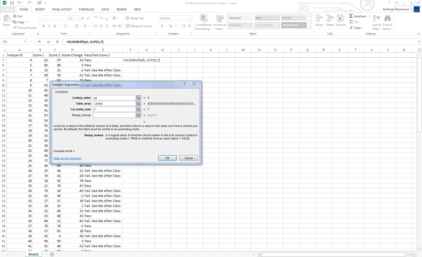
Vlookup
Vlookup is the power tool every Excel user should know. It helps you
herd data that's scattered across different sheets and workbooks and
bring those sheets into a central location to create reports and
summaries.
Vlookup helps you find information in large data tables such as inventory lists.
Say you work with products in a retail store. Each product typically
has a unique inventory number. You can use that as your reference point
for Vlookups. The Vlookup formula matches that ID to the corresponding
ID in another sheet, so you can pull information like an item
description, price, inventory levels, and other data points into your
current workbook.
Summon the Vlookup formula in the formula menu and enter the cell
that contains your reference number. Then enter the range of cells in
the sheet or workbook from which you need to pull data, the column
number for the data point you’re looking for, and either “True” (if you
want the closest reference match) or “False” (if you require an exact
match).
Creating charts
To create a chart, enter data into Excel with column headers, then select Insert > Chart > Chart Type. Excel 2013 even includes a Recommended Charts
section with layouts based on the type of data you’re working with.
Once the generic version of that chart is created, go to the Chart Tools menus to customize it. Don't be afraid to play around in here—there are a surprising number of options.
Excel 2013 includes Recommended Charts with layouts based on the type of data you're working with.
IF formulas
IF and IFERROR are the two most useful IF formulas in Excel. The IF
formula lets you use conditional formulas that calculate one way when a
certain thing is true, and another way when false. For example, you can
identify students who scored 80 points or higher by having the cell
report “Pass” if the score in column C is above 80, and “Fail” if it’s
79 or below.
IF formulas let you pull in just the data you need.
IFERROR is a variant of the IF Formula. It lets you return a certain
value (or a blank value) if the formula you’re trying to use returns an
error. If you’re doing a Vlookup to another sheet or table, for example,
the IFERROR formula can render the field blank if the reference is not
found.
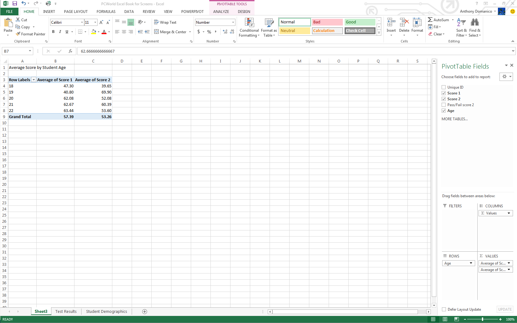
PivotTables
PivotTables are essentially summary tables that let you count,
average, sum, and perform other calculations according to the reference
points you enter. Excel 2013 added Recommended PivotTables, making it even easier to create a table that displays the data you need.
To create a PivotTable manually, ensure your data is titled appropriately, then go to Insert > PivotTable
and select your data range. The top half of the right-hand-side bar
that appears has all your available fields, and the bottom half is the
area you use to generate the table.
PivotTables are a summarization tool that let you perform calculations according to the reference points you enter.
For example, to count the number of passes and fails, put your Pass/Fail column into the Row Labels tab, then again into the Values
section of your PivotTable. It will usually default to the correct
summary type (count, in this case), but you can choose among many other
functions in the Values dropdown box. You can also create subtables that summarize data by category—for example, Pass/Fail numbers by gender.
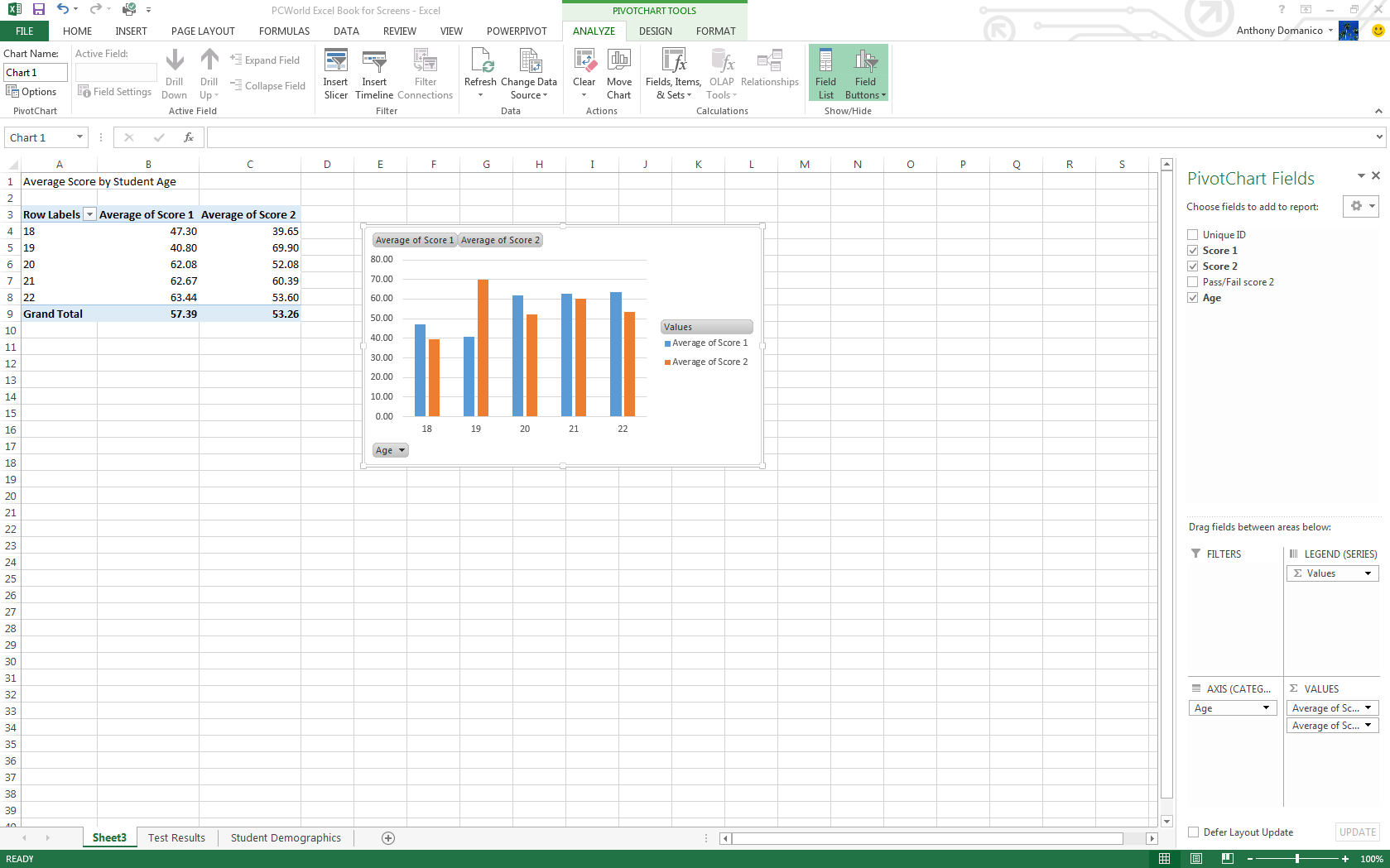
PivotChart
Part PivotTable, part traditional Excel chart, a PivotChart lets you
quickly and easily look at complex data sets in an easy-to-digest way.
PivotCharts have many of the same functions as traditional charts, with
data series, categories, and the like, but they add interactive filters
so you can browse through data subsets.
PivotCharts help you easily digest complex data.
Excel 2013 added Recommended PivotCharts, which can be found under the Recommended Charts icon in the Charts area of the Insert
tab. You can preview a chart by hovering your mouse over that option.
You can also manually create a PivotChart by selecting the PivotChart icon on the Insert tab..
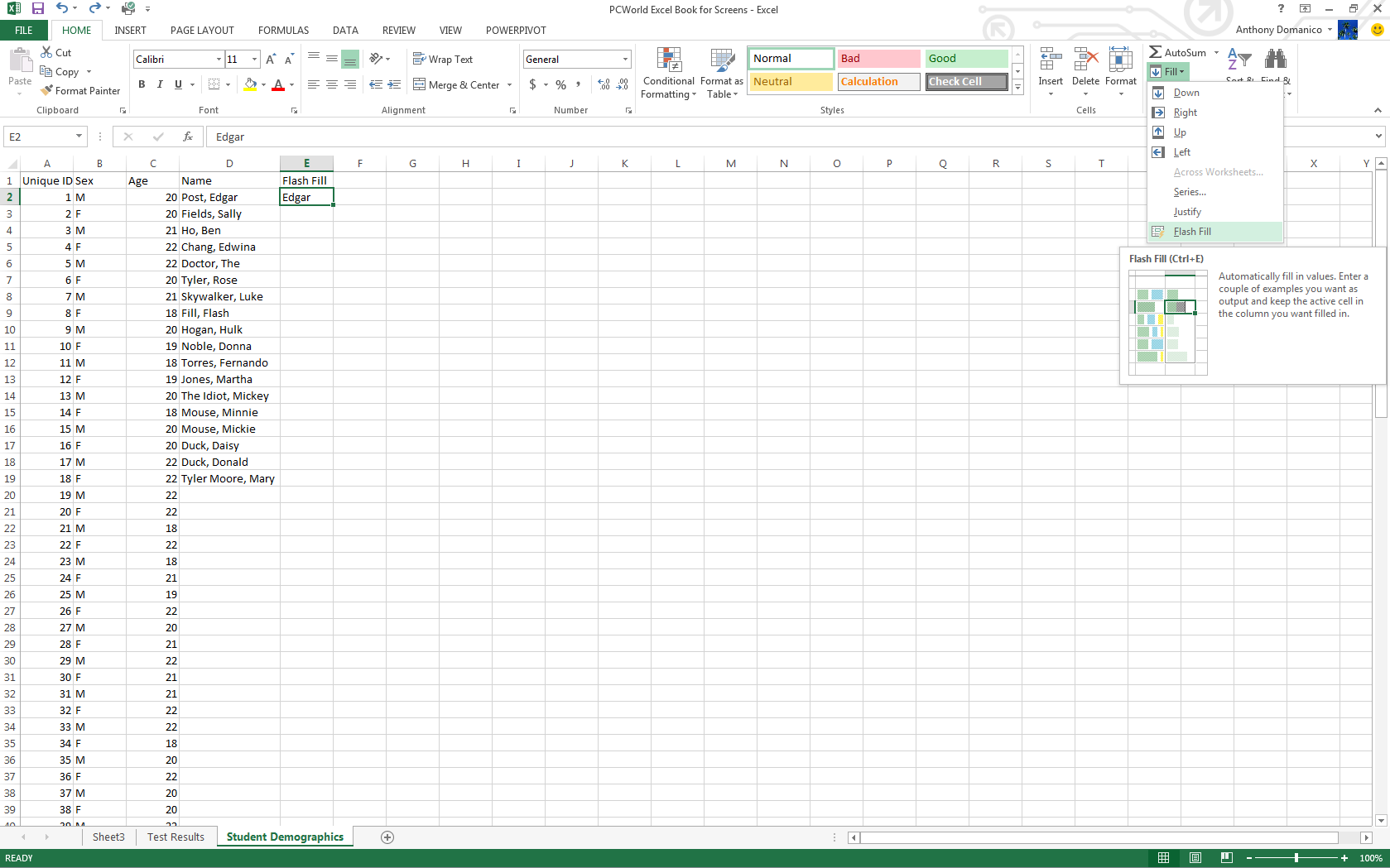
Flash Fill
Easily the best new feature
in Excel 2013, Flash Fill solves one of the most frustrating problems
of Excel: pulling needed pieces of information from a concatenated cell.
When you’re working in a column with names in “Last, First” format, for
example, you historically had to either type everything out manually or
create an often-complicated workaround.
Flash Fill can automtically add data formatted the way you want without using formulas.
In Excel 2013, you can now just type the first name of the first
person in a field immediately next to the one you’re working on, and
click Home > Fill > Flash Fill, and Excel will automagically extract the first name from the remaining people in your table.
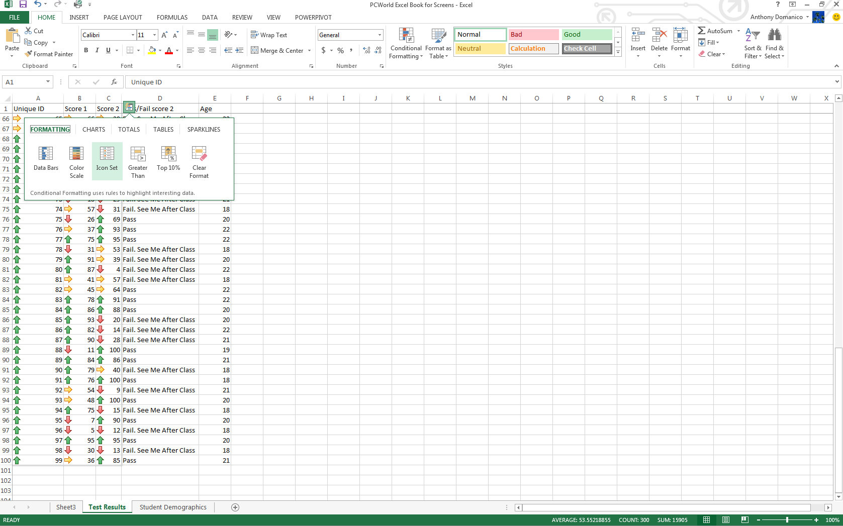
Quick Analysis
Excel 2013’s new Quick Analysis tool minimizes the time needed to
create charts based on simple data sets. Once you have your data
selected, an icon appears in the bottom right hand corner that, when
clicked, brings up the Quick Analysis menu.
Quick Analysis speeds the process of working with simple data sets.
This menu provides tools like Formatting, Charts, Totals, Tables, and Sparklines. Hovering your mouse over each one generates a live preview.
Power View
Power View is an interactive data exploration and visualization tool
that can pull and analyze large quantities of data from external data
files. Go to Insert > Reports in Excel 2013.
Power View creates interactive, presentation-ready reports.
Reports created with Power View are presentation-ready with reading
and full-screen presentation modes. You can even export an interactive
version into PowerPoint. Several tutorials on Microsoft’s site will help you become an expert in no time.
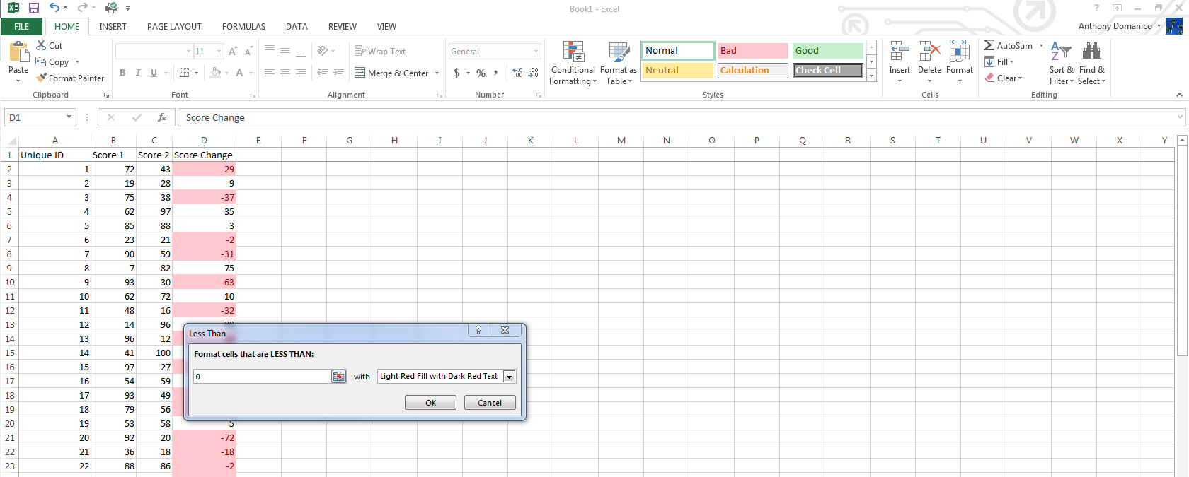
Conditional Formatting
For most tables, Excel’s extensive conditional formatting
functionality lets you easily identify data points of interest. Find
this feature on the Home tab in the taskbar. Select the range of cells you want to format, then click the Conditional Formatting dropdown. The features you’ll use most often are in the Highlight Cells Rules submenu.
Conditional Formatting lets you easily highlight data points of interest.
For example, say you’re scoring tests for your students and want to
highlight in red those whose scores dropped significantly. Using the Less Than conditional format, you can format cells that are less than -20 (a 20-point drop) with the Red Text or Light Red Fill with Dark Red Text
function. You can create many different kinds of rules, with unlimited
formats available via the custom format function within each item.
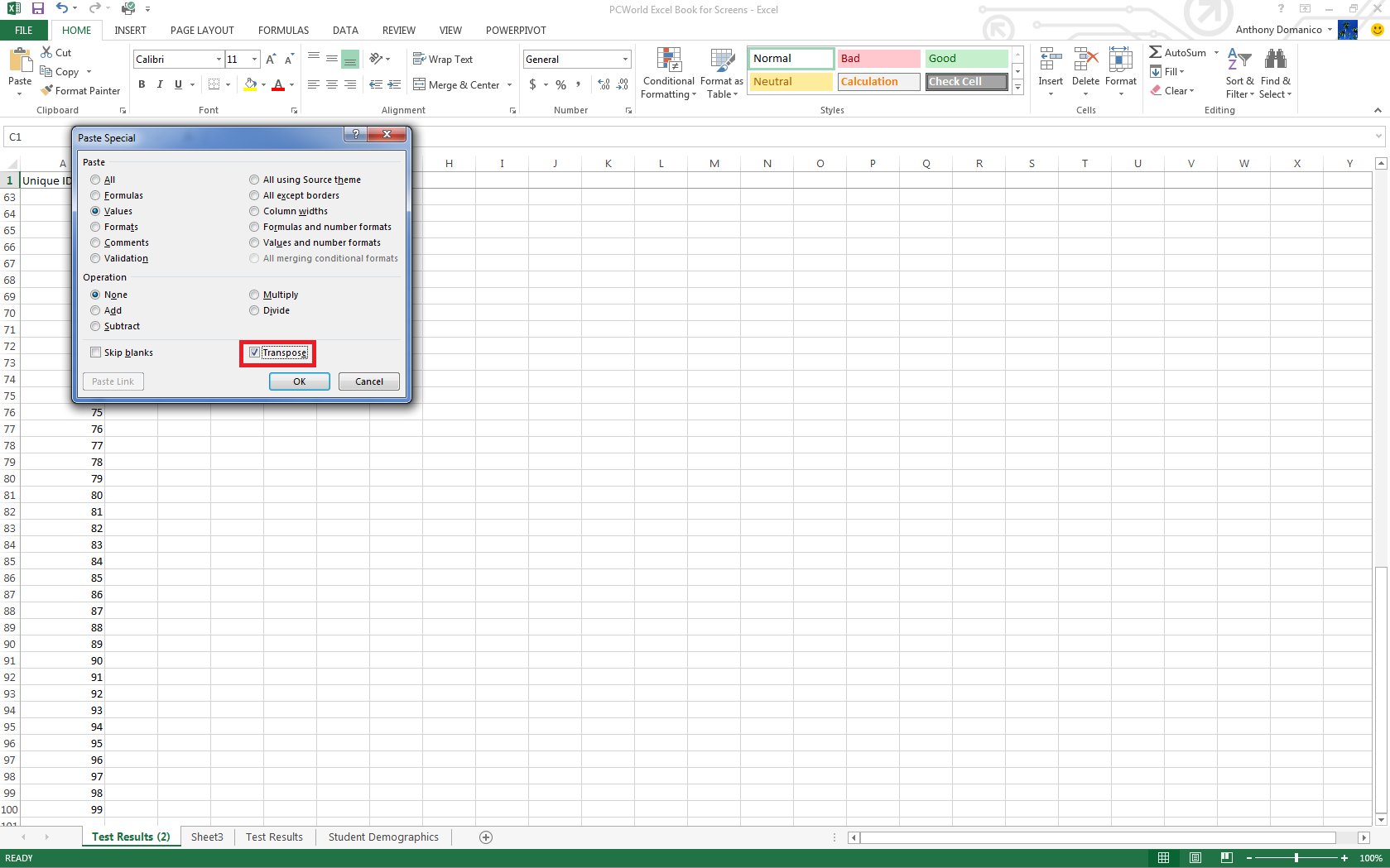
Transposing columns into rows (and vice versa)
Sometimes you’ll be working with data formatted in columns and you
really need it to be in rows (or the other way around). Simply copy the
row or column you’d like to transpose, right click on the destination
cell and select Paste Special. A checkbox on the bottom of the resulting popup window is labeled Transpose. Check the box and click OK. Excel will do the rest.
The Paste Special feature transposes columns and rows.
 Record a macro