There are three key elements of Six Sigma Process Improvement.
Customers
Processes
Employees
The Customer:
Customers define quality. They expect performance, reliability,
competitive prices, on-time delivery, service, clear and correct
transaction processing and more.
Today, Delighting a customer is a necessity. Because if we don't do it, someone else will!
The Processes:
Defining Processes and defining Metrics and Measures for Processes is the key element of Six Sigma.
Quality requires to look at a business from the customer's
perspective, In other words, we must look at defined processes from the
outside-in.
By understanding the transaction lifecycle from the customer's needs
and processes, we can discover what they are seeing and feeling. This
will give a chance to identify week area with in a process and then we
can improve them.
To watch calculations results immediately:
1. Select range of cells containing numeric data.
2. Select the Status Bar and right-click to open Status Bar shortcut menu.
Six functions are available:
Average, Count, Numerical Count, Minimum, Maximum and Sum
Results appear at the right of each formula in the shortcut menu.
Or
Check all or any other formulas you want to watch the result calculation for in the Status Bar.
The following articles are available for the 'Worksheet Functions' topic. Click the article's title (shown in bold) to see the associated article.
Calculating Fractions of Years When
working with dates and the relationship between dates, Excel provides a
variety of worksheet functions that may prove helpful. One such
function is YEARFRAC, which allows you to calculate what fraction of a
year is represented by the number of days between two dates.
Converting Strings to Numbers When
working with data in a macro, there are two broad categories you can
manipulate: numbers and text. Sometimes you need to convert information
from one category (data type) to another. Here is how you convert text
to numbers.
Converting to Hexadecimal Excel
allows you to easily convert values from decimal to other numbering
systems, such as hexadecimal. This tip explains how to use the DEC2HEX
worksheet function.
Converting to Octal If
you need to do some work in the base-8 numbering system (octal), you'll
love two worksheet functions provided by Excel for this purpose. These
functions allow you to convert values to octal and convert them back
again.
Counting Displayed Cells When
you filter data, Excel displays only a portion of what is really in a
worksheet. If you want to count the number of cells that are displayed
after filtering, then you'll want to explore the techniques in this tip.
Counting Unique Values with Functions Using
Excel to maintain lists of information is not unusual. When working
with the list you may need to determine how many unique values it
contains. This tip shows you how.
Functions Within Functions Functions
are the heart of Excel's power. The program allows you to compound that
power by handily putting one function inside another function.
Iterating Circular References Does
your data require that you perform calculations using circular
references? If so, then you'll want to be aware of the way in which
Excel handles those references.
Numbers in Base 12 Different
professions use numbers in entirely unique ways. You may need to come
up with a number that represents the number of 12-unit groupings. This
tip examines a way this can be done.
Random Numbers in a Range Excel
provides several different functions that you can use to generate
random numbers. One of the most useful is the RANDBETWEEN function,
which allows you to generate a random number between a lower and upper
boundary that you specify.
Returning a Blank Value Is
it possible for a formula to return a blank value? It depends on how
you define your terms. This tip examines all the ins and outs of
returning "nothing" from a formula and how that affects some of the more
common worksheet functions.
Selecting Random Names Got
a tone of names from which you need to select a few random names? There
are several ways you can extract what you need; several different ideas
are explained in this tip.
Understanding Functions Excel uses Functions to assist in creating spreadsheets that perform a multitude of calculations.
Using the WEEKNUM Function Need
to know which week of the year a particular date falls within? Excel
provides the WEEKNUM function so you can easily calculate this
statistic.
Working with Roman Numerals Understanding and using a function to replace an Arabic number with Roman numerals. And, as a bonus, how to change them back.
Keyboard shortcuts are the best way to navigate cells or enter formulas more quickly. We’ve listed our favorites below. Control-Down/Up Arrow = Moves to the top or bottom cell of the current column Control-Left/Right Arrow = Moves to the cell furthest left or right in the current row Control-Shift-Down/Up Arrow = Selects all the cells above or below the current cell Shift-F11 = Creates a new blank worksheet within your workbook F2 = opens the cell for editing in the formula bar Control-Home = Navigates to cell A1 Control-End = Navigates to the last cell that contains data Alt-= = Autosums the cells above the current cell
Excel is arguably one of the best programs ever made, and it has
remained the gold standard for nearly all businesses worldwide. But
whether you’re a newbie or a power user, there's always something left
to learn. Or do you think you've seen it all and done it all? Let us
know what we've missed in the comments.
There are two kinds of Microsoft Excel
users in the world: Those who make neat little tables, and those who
amaze their colleagues with sophisticated charts, data analysis, and
seemingly magical formula and macro tricks. You, obviously, are one of
the latter—or are you? Check our list of 11 essential Excel skills to
prove it—or discreetly pick up any you might have missed.
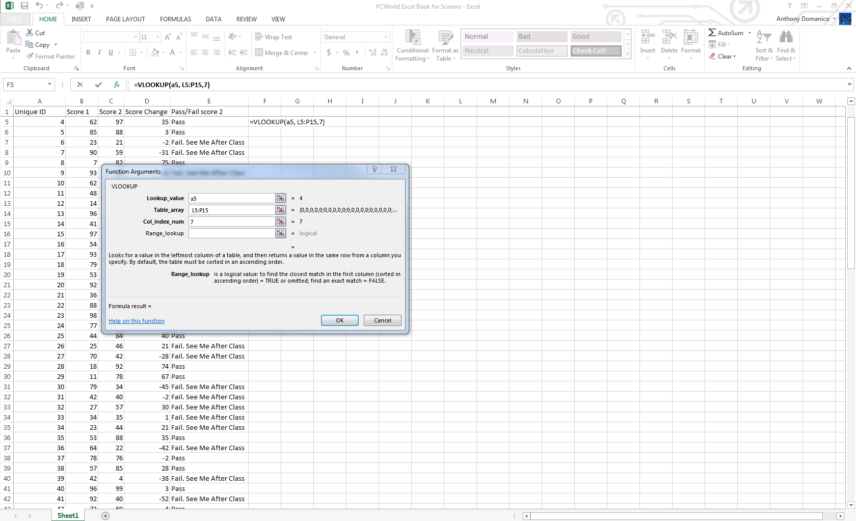
Vlookup
Vlookup is the power tool every Excel user should know. It helps you
herd data that's scattered across different sheets and workbooks and
bring those sheets into a central location to create reports and
summaries.
Vlookup helps you find information in large data tables such as inventory lists.
Say you work with products in a retail store. Each product typically
has a unique inventory number. You can use that as your reference point
for Vlookups. The Vlookup formula matches that ID to the corresponding
ID in another sheet, so you can pull information like an item
description, price, inventory levels, and other data points into your
current workbook.
Summon the Vlookup formula in the formula menu and enter the cell
that contains your reference number. Then enter the range of cells in
the sheet or workbook from which you need to pull data, the column
number for the data point you’re looking for, and either “True” (if you
want the closest reference match) or “False” (if you require an exact
match).
Creating charts
To create a chart, enter data into Excel with column headers, then select Insert > Chart > Chart Type. Excel 2013 even includes a Recommended Charts
section with layouts based on the type of data you’re working with.
Once the generic version of that chart is created, go to the Chart Tools menus to customize it. Don't be afraid to play around in here—there are a surprising number of options.
Excel 2013 includes Recommended Charts with layouts based on the type of data you're working with.
IF formulas
IF and IFERROR are the two most useful IF formulas in Excel. The IF
formula lets you use conditional formulas that calculate one way when a
certain thing is true, and another way when false. For example, you can
identify students who scored 80 points or higher by having the cell
report “Pass” if the score in column C is above 80, and “Fail” if it’s
79 or below.
IF formulas let you pull in just the data you need.
IFERROR is a variant of the IF Formula. It lets you return a certain
value (or a blank value) if the formula you’re trying to use returns an
error. If you’re doing a Vlookup to another sheet or table, for example,
the IFERROR formula can render the field blank if the reference is not
found.
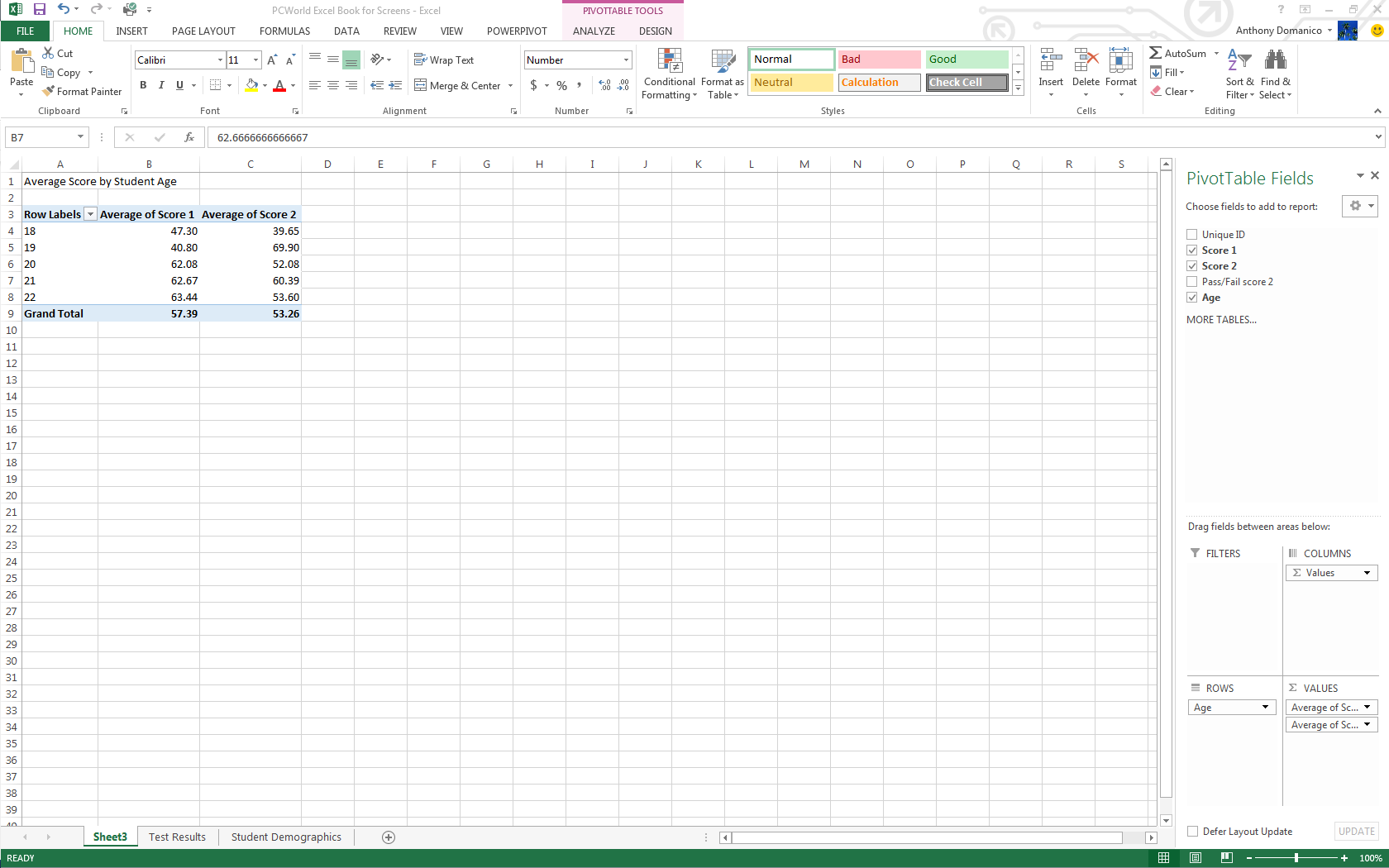
PivotTables
PivotTables are essentially summary tables that let you count,
average, sum, and perform other calculations according to the reference
points you enter. Excel 2013 added Recommended PivotTables, making it even easier to create a table that displays the data you need.
To create a PivotTable manually, ensure your data is titled appropriately, then go to Insert > PivotTable
and select your data range. The top half of the right-hand-side bar
that appears has all your available fields, and the bottom half is the
area you use to generate the table.
PivotTables are a summarization tool that let you perform calculations according to the reference points you enter.
For example, to count the number of passes and fails, put your Pass/Fail column into the Row Labels tab, then again into the Values
section of your PivotTable. It will usually default to the correct
summary type (count, in this case), but you can choose among many other
functions in the Values dropdown box. You can also create subtables that summarize data by category—for example, Pass/Fail numbers by gender.
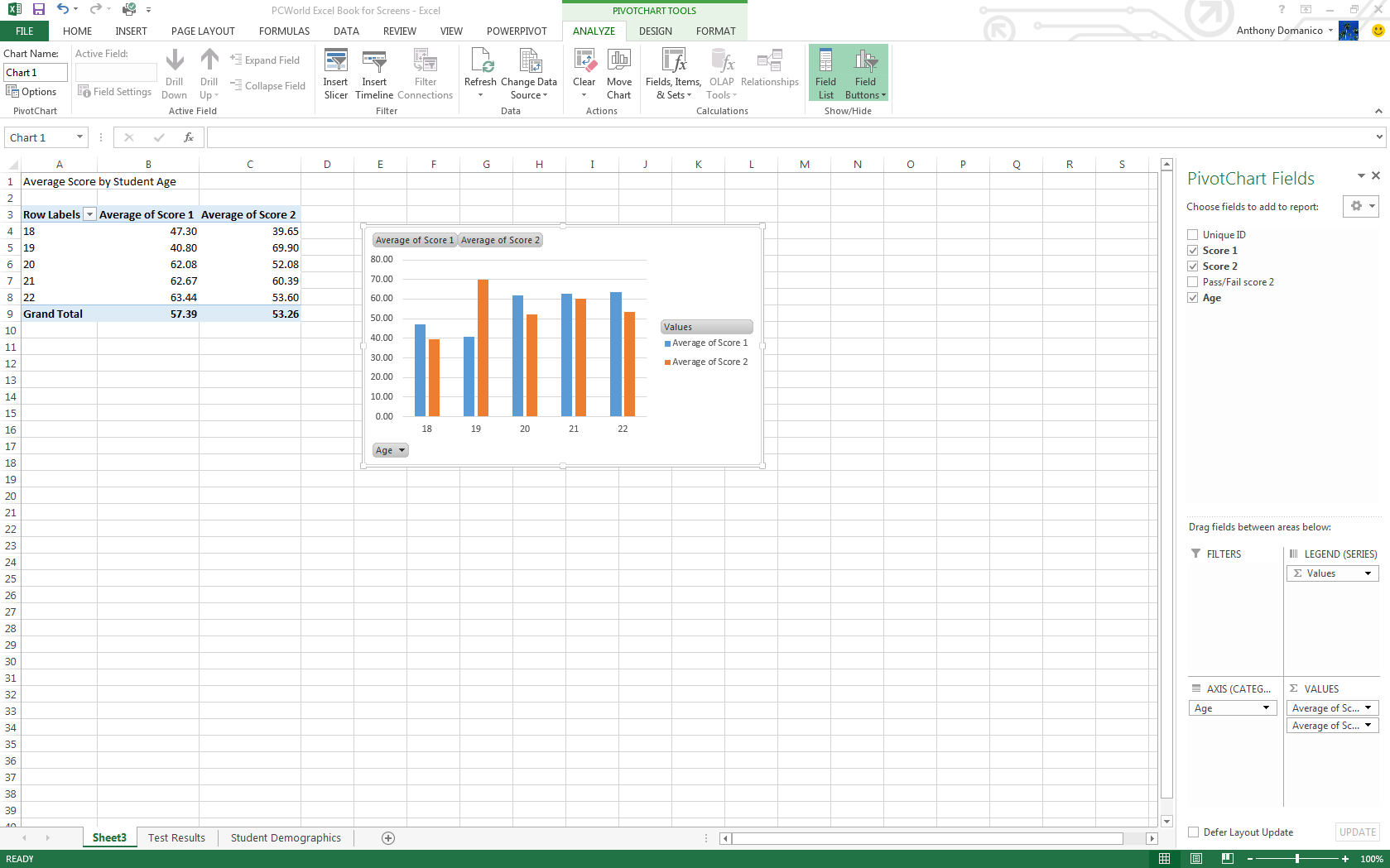
PivotChart
Part PivotTable, part traditional Excel chart, a PivotChart lets you
quickly and easily look at complex data sets in an easy-to-digest way.
PivotCharts have many of the same functions as traditional charts, with
data series, categories, and the like, but they add interactive filters
so you can browse through data subsets.
PivotCharts help you easily digest complex data.
Excel 2013 added Recommended PivotCharts, which can be found under the Recommended Charts icon in the Charts area of the Insert
tab. You can preview a chart by hovering your mouse over that option.
You can also manually create a PivotChart by selecting the PivotChart icon on the Insert tab..
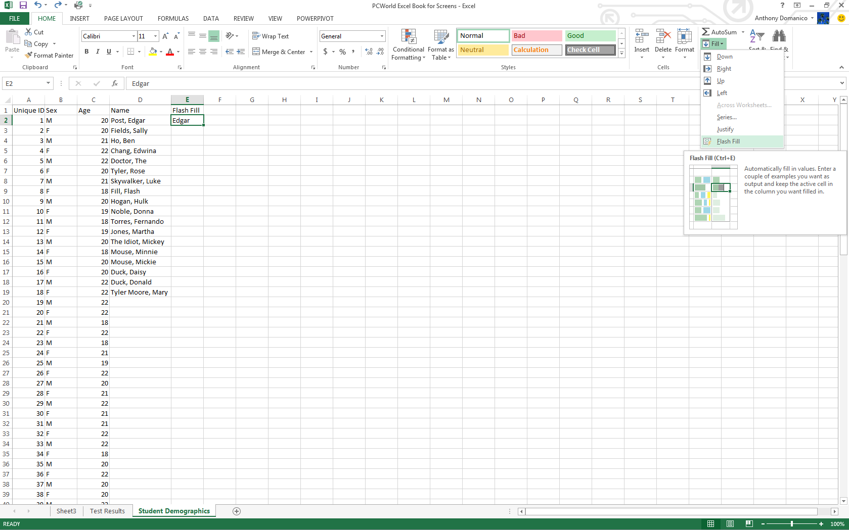
Flash Fill
Easily the best new feature
in Excel 2013, Flash Fill solves one of the most frustrating problems
of Excel: pulling needed pieces of information from a concatenated cell.
When you’re working in a column with names in “Last, First” format, for
example, you historically had to either type everything out manually or
create an often-complicated workaround.
Flash Fill can automtically add data formatted the way you want without using formulas.
In Excel 2013, you can now just type the first name of the first
person in a field immediately next to the one you’re working on, and
click Home > Fill > Flash Fill, and Excel will automagically extract the first name from the remaining people in your table.
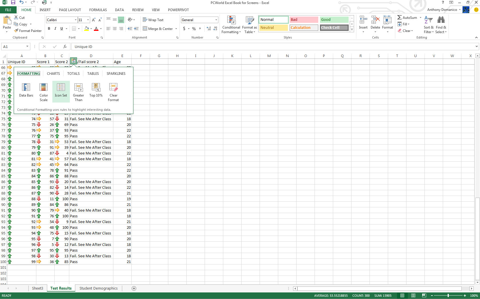
Quick Analysis
Excel 2013’s new Quick Analysis tool minimizes the time needed to
create charts based on simple data sets. Once you have your data
selected, an icon appears in the bottom right hand corner that, when
clicked, brings up the Quick Analysis menu.
Quick Analysis speeds the process of working with simple data sets.
This menu provides tools like Formatting, Charts, Totals, Tables, and Sparklines. Hovering your mouse over each one generates a live preview.
Power View
Power View is an interactive data exploration and visualization tool
that can pull and analyze large quantities of data from external data
files. Go to Insert > Reports in Excel 2013.
Power View creates interactive, presentation-ready reports.
Reports created with Power View are presentation-ready with reading
and full-screen presentation modes. You can even export an interactive
version into PowerPoint. Several tutorials on Microsoft’s site will help you become an expert in no time.
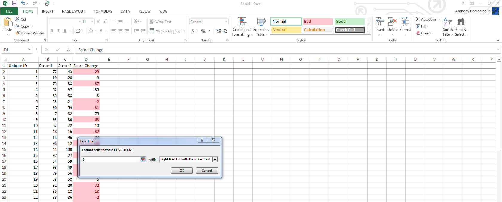
Conditional Formatting
For most tables, Excel’s extensive conditional formatting
functionality lets you easily identify data points of interest. Find
this feature on the Home tab in the taskbar. Select the range of cells you want to format, then click the Conditional Formatting dropdown. The features you’ll use most often are in the Highlight Cells Rules submenu.
Conditional Formatting lets you easily highlight data points of interest.
For example, say you’re scoring tests for your students and want to
highlight in red those whose scores dropped significantly. Using the Less Than conditional format, you can format cells that are less than -20 (a 20-point drop) with the Red Text or Light Red Fill with Dark Red Text
function. You can create many different kinds of rules, with unlimited
formats available via the custom format function within each item.
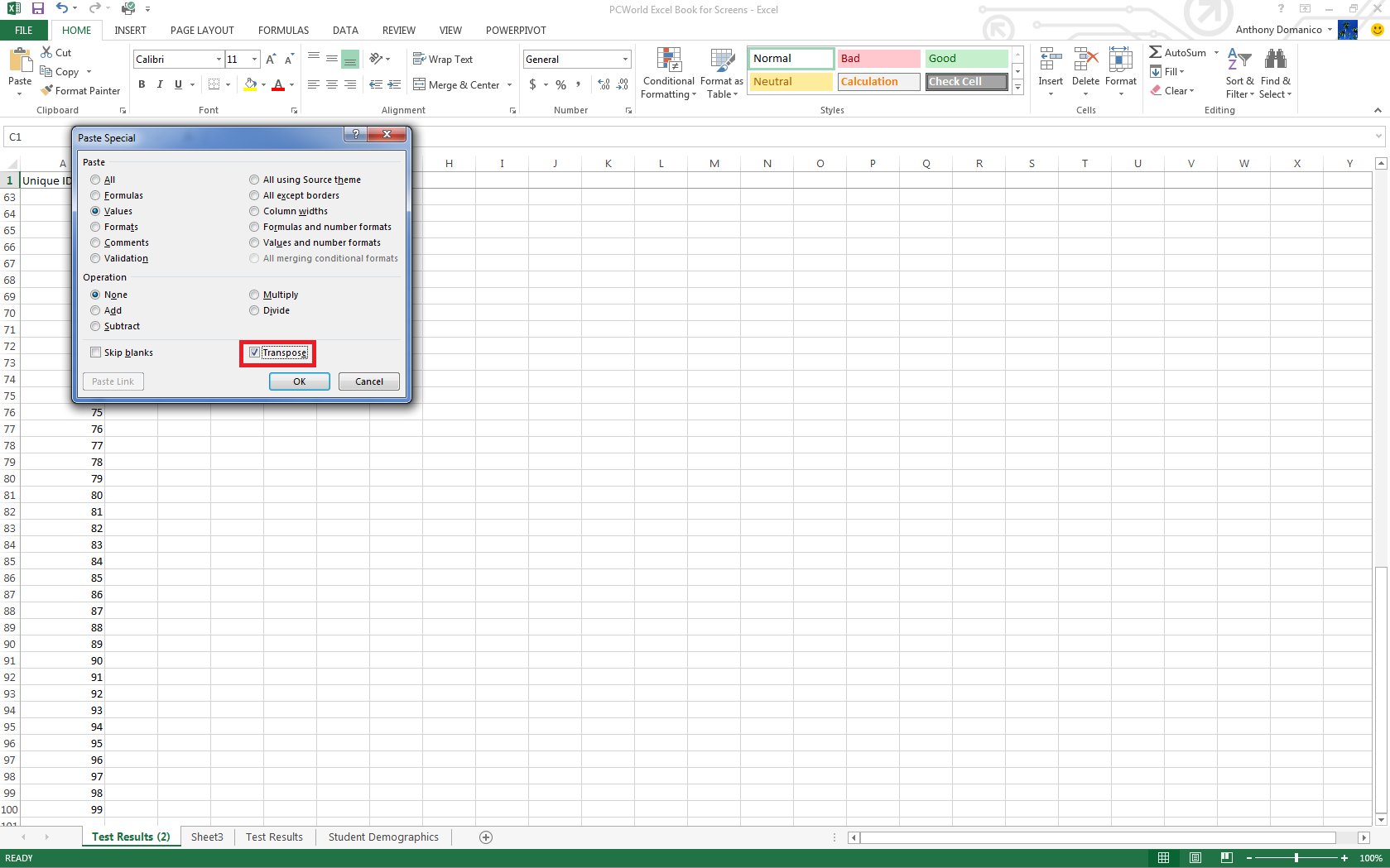
Transposing columns into rows (and vice versa)
Sometimes you’ll be working with data formatted in columns and you
really need it to be in rows (or the other way around). Simply copy the
row or column you’d like to transpose, right click on the destination
cell and select Paste Special. A checkbox on the bottom of the resulting popup window is labeled Transpose. Check the box and click OK. Excel will do the rest.
The Paste Special feature transposes columns and rows.